A. Lab Goals

• You will learn about the operation of unclocked memory circuits and you will construct and test an electronic lock with two level input signals and two output signals.
  
  
• Although you won't have to design an electronic lock for this lab, you will have to be familiar with the basic concepts to adequately analyze the circuit operation.

B. Background Reading

• This information can be found in sections 10.4 - 10.6 in (N/N) or chapter 9 in (M).
  
  
• Make certain that you are familiar with the concepts of excitation tables, cycles, stable and unstable states, etc.

C. Definitions

• Asynchronous sequential circuit
  
  
• Cycle
  
  
• Diode
  
  
• Excitation table
  
  
• Flow table
  
  
• Fundamental-mode circuit
  
  
• LED
  
  
• Level input
  
  
• Primitive flow table
  
  
• Pulse-mode circuit
  
  
• Race condition
  
  
• Secondary state
  
  
• Unstable state

D. Laboratory Equipment

• No new equipment for this lab. An ooscilloscope may be used to measure rise times and verify delays. A DLA may be used to plot the time dependence of the states for specific input sequences.

E. New Hardware

• No new hardware is requred for this lab.

F. Circuit Analysis

• In this section we will analyze the simple asynchronous sequential circuit shown in Fig. 8.1 with two inputs X₁ and X₂ and a single excitation state Y.
  
  
  
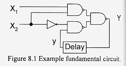
• In this example, Y also functions at the desired output state, but in general you could have separate outputs that are not used in any feedvack loop.
  
  
• The excitation signal is fed back to the inputs of the logic gates either directly, or through some circuitry which has an assocated delay as indicated in the figure.
  
  
• We call the feedback signal a secondary state and we consider the total state of the circuit to consist of both the independent input states and the secondary states.
  
  
• For our example the total state for the circuit in Fig. 8.1 is the set {X₁, X₂, y}.
  
  
• We use a lower case symbol (y) to represent the secondary state in order to emphasize the fact that there is a time lag in the circuit and that y is determined by Y at some earlier time.
  
  
• The feedback increases the complexity of the circuit analysis.
  
  
• When Y changes states, the feedback signal will subsequently change some of the values of the gate inputs, and those changes may in turn change the excitation state, which will results in a change of the gate inputs and so on.
  
  
• When a change to the secondary state produces a subsequent change to the excitation state, we say that the state is unstable.
  
  
• A state is stable if a change to the secondary state produces no further change to the excitation state.
  
  
• This means that the output state will remain constant, at least until there are additional changes to the level inputs.
  
  
  
• We will now examine the operation of the fundamental-mode circuit shown in Fig. 8.1.
  
  
• The procedure that we will use to characterize the operation of the circuit will be the same procedure that you will use when you are preparing for the lab.
  
  
• By fundamental-mode circuit, we mean to say that we have level inputs and that only one input level can be chaged at any given time.
  
  
• The first step in the analysis is to create an excitation (state) table just as we have done in the analysis of synchronous sequential circuits.
  
  
• We put the values of the excitation state in our table as a function of the total state.
  
  
• We can quickly find the expression for the excitation state in terms of the total state to be:
  
  Y = ((X₁X₂)'(yX₂')' = X₁X₂ + yX₂'.
  
  
  
• The excitation table which corresponds to the function given in the previous line is given in Fig. 8.2.
  
  
  
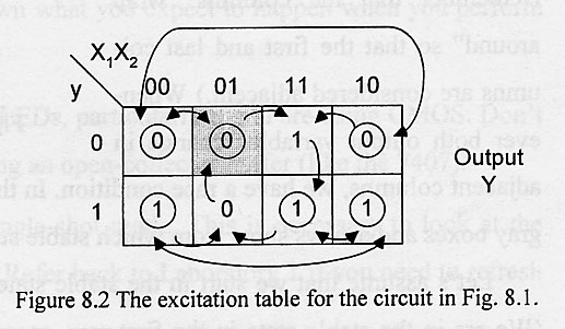
• The stable states are indicated by the circles in the table.
  
  
• Let's use this table to figure out how the experiment would go if we were to build and test this circuit.
  
  
• Let's say that we initially had an input of X₁X₂ = 01 and that we were in the state Y = 0.
  
  
• This is a stable state because the secondary state is also zero.
  
  
• We are not allowed to changhe the input to 10, because that would nmean that we simultaneously changed two inputs.
  
  
• Instead, we can go either to 00 or to 11.
  
  
• If we go to 00, the output remains at zero, so we staty in a new stable state.
  
  
• We can then transition to 10, whereby the output still remains zero, and we are in yet another stable state.
  
  
• Only when we transition to the input 11 when the output is zero, do we finally reach an unstable state, because the excitation state changes to 1.
  
  
• The secondary state will follow to 1 and we will move to the stable state on the bottom row.
  
  
• From an input of 11 and an output of 1, if we change the input to 01, we will hit another unstable state and move up again to the top row.
  
  
• If instead we had moved to an input of 10, we would have been in a stable state.
  
  
  
• With only one state variable we don't have to worry about race conditions.
  
  
• However, with two or more secondary states there is a real possibility of developing a circuit with critical race condition.
  
  
  
• The race conditions are easily found by looking at the table.
  
  
  
• Changing input values means that we move from one coumn to the next in the same row.
  
  
• Since we can only change one input variable at a time, we oncentrate on adjacent row members.
  
  
• Whenever both output vaiables change in adjacent couums, we have a race condition.
  
  
• In this table, the race conditions are indicated by the gray boxes and arrows show from which stable states we can initiate these race conditions.
  
  
  
• Let's assume that we start in the stable state 0100, i.e., the input is 01 and the output is 00.
  
  
• If we change the input to 11, both output states try to change from zero to one.
  
  
• If the change could occur simultaneously, we would end up in the stable state 1111.
  
  
• However, in reality, one output will change before the other, and we may not end up in the desired state.
  
  
• The only way to discover if the race is critical is to first assume Y₁ changes first and see where we end up.
  
  
• Then we assume Y₂ changes first and see where we end up.
  
  
• If we end up in the correct place regardless of the assumption, we found a non-critical race.
  
  
• It turns out that all the races in this "circuit" are critical.
  
  
  
  
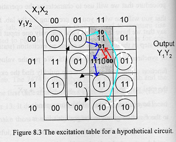
• If Y₁ changes first, the secondary state goes from 00 to 10, which is equal to the excitation state, so we end up in a stable state.
  
  
• We were "supposed" to switch to the 11 state, but erroneously we are in the 10 state.
  
  
• However, if Y₂ chages first, the secondary state goes to 01, and the output tries to transition to 10, which means we have another race condition.
  
  
• Again we have to look at two different cases.
  
  
• If Y₁ changes first, we go to a secondary state of 11, which is stable.
  
  
• This is where we originallhy wanted to be.
  
  
• If Y₂ changes first, we go to the secondary state 00, which is where we started.
  
  
• The output would then try to change to 11 and we would oscillate.
  
  
• We may end up in the correct state, we may end up in the wrong state, or the circuit may oscillate!
  
  
  
• As a final example, let's look at a cycle transition.
  
  
• Assume that we start in the total state 1111 and we change the input to 01.
  
  
• That puts us in the unstable state 0111, which transitrions us to the unstable state 0110, which finally transitions us to the stable state 0100.
  
  
• The definition of a cycle is that we go through two or more unstable states, but it doesn't necessarily mean trouble!

Laboratory 8 Description

Objective:

• To learn about the design and operation of unclocked memory circuits; to construct and test the operation of an electronic lock with two level input signals and two output signals.
  
  
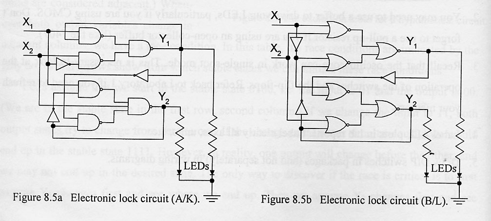
• You will do lab 8B (TTL, Fig. 8.5b)
  
  
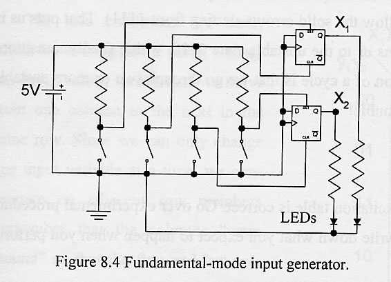
• Figure 8.4 shows the switches and the flip-flops are used to generate two input signals: X₁ (from the upper FF) and X₂ (from the lower FF).
  
  
• The output from Fig. 8.4 must be connected to the inputs for your lab.
  
  
  

  Available Hardware:

  Digital component boxes - See Appendix G.

  Pre-lab preparation

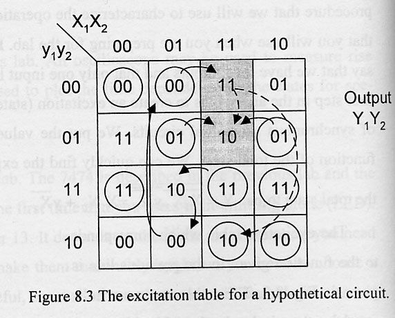
  As an example, we analyze the circuit shown in Fig. 8.5a.
  
  The expressions for the excitation states in terms of the total state are
  
  Y₁ = ((X₁y₁)'(X₁'X₂)')' = X₁y₁ + X₁'X₂
  
  and
  
  Y₂ = ((X₁y₂')'(y₁'y₂)'X₂)' = X₁y₂' + y₁'y₂ + X₂'.
  
  The excitation table is found as
  
  

  		X1X2
  		00	01	11	10	Y1	Y2
  y1y2	00	01	10	01	01	X1'X2	X1' + X2
  	01	01	11	01	01	X1'X2	1 + X2'
  	11	01	10	10	11	X1 + X1'X2	X2'
  	10	01	10	11	11	X1 + X1'X2	X1 + X2'

  
  
  
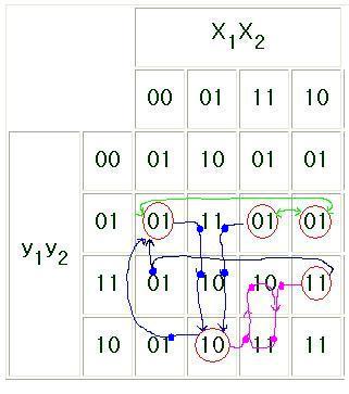
  We find: five stable modes, no race conditions, three cycles, and two ocillations.
  
  Part I - manual operation
  Part II - repetitive operation
  
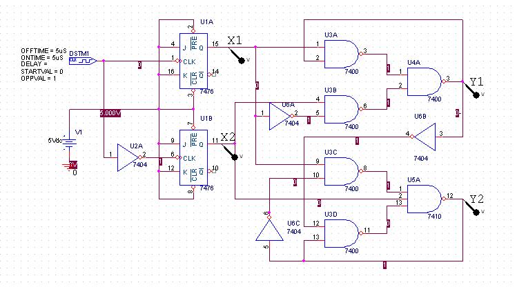
  Schematic diagram
  
  
  
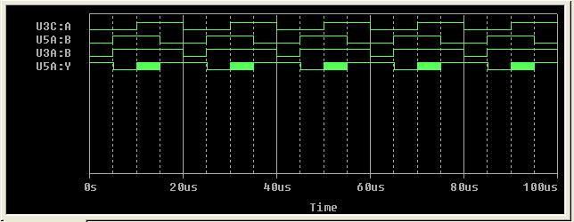
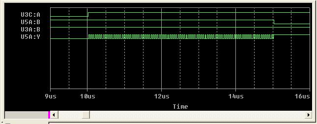
  Plots of X₁(U3C:A), X₂U5A:B), Y₁(U3A:B), and Y₂(U5A:Y)
  
  

  Experimental Procedure:

  During this experiment, be certain that you:
  • Ask the TA questions regarding any procedures about which you are uncertain.
    
    
  • Turn off all power supplies any time that you make any change to the circuit.
    
    
  • Do NOT apply more that 5 V to the circuit at any time.
    
    
  • Arrange your circuit components neatly and in a logical order.
    
    
  • Compare your breadboards carefully with your circuit diagrams before applying power to the circuit.
    
    
  • Complete the following tasks:
    • Part I - manual operation
      
    • Part II - repetitive operation
      
    • Part III - excitation table verification
      

    Post-lab analysis:

    Generate a lab report following the sample report available in Appendix A. Mention any difficulties encountered during the lab. Describe any results that were unexpected and try to accoundt for the origin of these results(i.e. explain what happened). In ADDITION, answer the following questions:
    
    • Part I - manual operation
      
    • Part II - repetitive operation